Machine learning is susceptible to poisoning attacks, in which an attacker controls a small fraction of the training data and chooses that data with the goal of inducing some behavior (unintended by the model developer) in the trained model . Previous works have mostly considered two extreme attacker objectives: indiscriminate attacks, where the attacker's goal is to reduce overall model accuracy , and instance-targeted attacks, where the attacker's goal is to reduce accuracy on a specific known instance . Recently, Jagielski et al. introduced the subpopulation attack, a more realistic setting in which the adversary attempts to control the model’s behavior on a specific subpopulation while having negligible impact on the model’s performance on the rest of the population. Such attacks are more realistic — for example, the subpopulation may be a type of malware produced by the adversary that they wish to have classified as benign, or a type of demographic individual for which they want to increase (or decrease) the likelihood of being selected by an employment screening model — and are harder to detect than indiscriminate attacks.

In this article, we present visualizations to understand poisoning attacks in a simple two-dimensional setting, and to explore a question about poisoning attacks against subpopulations of a data distribution: how do subpopulation characteristics affect attack difficulty? We visually explore these attacks by animating a poisoning attack algorithm in a simplified setting, and quantifying the difficulty of the attacks in terms of the properties of the subpopulations they are against.

Datasets for Poisoning Experiments

We study poisoning attacks against two different types of datasets: synthetic and tabular benchmark.

Synthetic datasets are generated using dataset generation algorithms from Scikit-learn and resemble Gaussian mixtures with two components. Each of these datasets is controlled by a set of parameters, which captures different global dataset properties. The first dataset parameter is the class separation parameter $\alpha \ge 0$ which controls the distance between the two class centers. The second dataset parameter is the label noise parameter $\beta \in [0, 1]$ which controls the fraction of points whose labels are randomly assigned. The reason for varying the dataset parameters in our experiments is to determine how properties of the dataset affect poisoning attack difficulty. The synthetic datasets are limited to just two features, so that direct two-dimensional visualizations of the attacks are possible.

We also perform poisoning attacks against the UCI Adult dataset , which has been used previously in the evaluations of subpopulation poisoning attacks . The Adult dataset is of much higher dimension (57 after data transformations), and so the attack process cannot be visualized directly as in the case of synthetic datasets. The purpose of this dataset is to gauge the attack behavior in a more realistic setting.

Synthetic Dataset Parameter Space

We generate synthetic datasets over a grid of the dataset parameters. For each combination of the two parameters, 10 synthetic datasets are created by feeding different random seeds.

We use linear SVM models for our experiments. Before conducting the poisoning attacks against the subpopulations, let’s observe the behavior of the clean models trained on each combination of the dataset parameters:

The overall trends in the plot meet our expectation: clean model accuracy improves as the classes become more separated and exhibit less label noise.

Poisoning Attacks

We use the model-targeted poisoning attack design from Suya et al. , which is shown to have state-of-the-art performance on subpopulation attacks. In a model-targeted poisoning attack, the attacker's objective is captured in a target model and the attack goal is to induce a model as close as possible to that target model. By describing the attacker’s objective using a target model, complex objectives can be captured in a unified way and avoids the need of designing customized attacks for individual objectives. Since the attack is online, the poisoning points can be added into the training set until the attack objective is satisfied, giving a natural measure of the attack's difficulty in terms of the number of poisoning points added during the attack.

Our choice of attack algorithm requires a target model as input. For our attacks, the required target model is generated using the label-flipping attack variant described in Koh et al., which is also used by Suya et al. in their experiments. For each subpopulation, we use the label-flipping attack to generate a collection of candidate classifiers (using different fraction and repetition number) which each achieve 0% accuracy (100% error rate) on the target subpopulation. Afterwards, the classifier with the lowest loss on the clean training set is chosen to be the target model, as done in Suya et al..

For our case, the attack terminates when the induced model misclassifies at least 50% of the target subpopulation, measured on the test set. This threshold was chosen to mitigate the impact of outliers in the subpopulations. In earlier experiments requiring 100% attack success, we observed that attack difficulty was often determined by outliers in the subpopulation. By relaxing the attack success requirement, we are able to capture the more essential properties of an attack against each subpopulation. Since our eventual goal is to characterize attack difficulty in terms of the properties of the targeted subpopulation (which outliers do not necessarily satisfy), this is a reasonable relaxation.

Since we want to describe attack difficulties by the (essential) number of poisoning points needed (i.e., the number of poisoning points of the optimal attacks), more efficient attacks serve as better proxy to the (unknown) optimal poisoning attacks. To achieve the reported state-of-the-art performance using the chosen model-targeted attack, it is important to choose a suitable target model, and we ensure this by selecting the target models using the selection criteria mentioned above. This selection criteria is also justified in the analysis of the theoretical properties of the attack framework.

Synthetic Datasets

We use cluster subpopulations for our experiments on synthetic datasets. To generate the subpopulations for each synthetic dataset, we run the k-means clustering algorithm ($k=16$) and extract the negative-label instances from each cluster to form the subpopulations. Then, target models are generated according to the above specifications, and each subpopulation is attacked using the online (model-targeted) attack algorithm.

The above animation shows how the attack sequentially adds poisoning points into the training set to move the induced model towards the target model. Take note of how the poisoning points with positive labels work to reorient the model's decision boundary to cover the subpopulation while minimizing the impact on the rest of the dataset. This behavior also echoes with the target model selection criteria mentioned above, which aims to minimize the loss on the clean training set while satisfying the attacker goal. Another possible way to generate the target model is to push the entire clean decision boundary downwards without reorienting iti.e., the target model differs from the clean model only in the bias term., but this will result in a model with higher loss on other parts of the dataset, and thus a higher (overall) loss difference to the clean model. Intuitively, such an alternative would experience more "resistance" from the dataset, preventing the induced model from moving as swiftly to the target.

The above comparison demonstrates the importance of choosing a good target model and illustrates the benefits of the target model selection criteria above. By using a target model that minimizes the loss on the clean dataset, the attack algorithm is more likely to add poisoning points that directly contribute to the underlying attack objective. On the other hand, using a poor target model causes the attack algorithm to choose poisoning points that also attempt to preserve unimportant target model behaviors on other parts of the dataset.

Visualizations of Different Attack Difficulties

Now that we have described the basic setup for performing subpopulation poisoning attacks using the online attack algorithm, we can start to study specific examples of poisoning attacks in order to understand what affects their difficulties.

Easy Attacks with High Label Noise

Let's look at a low-difficulty attack. The below dataset exhibits a large amount of label noise $(\beta = 1)$, and as a result the clean model performs very poorly. When the poisoning points are added, the model is quickly persuaded to change its decision with respect to the target subpopulation.

In this particular example, there is a slight class imbalance due to dividing the dataset into train and test sets (963 positive points and 1037 negative points). As a result of this and the label noise, the clean model chooses to classify all points as the majority (negative) label.

One interesting observation in this example is, despite being easy to attack overall, attack difficulties of different subpopulations still vary somewhat consistently based on their relative locations to the rest of the dataset. Selecting other subpopulations in the animation reveals that subpopulations near the center of the dataset tend to be harder to attack, while subpopulations closer to the edges of the dataset are more vulnerable. This behavior is especially apparent with this subpopulation in the lower cluster, where the induced model ends up awkwardly wedged between the two clusters (now referring to the two main "clusters" composing the dataset).

Easy Attacks with Small Class Separation

The next example shows an attack result similar to the noisy dataset shown above, but now the reason of low attack difficulty is slightly different: although the clean training set now has small label noise, the model does not have enough capacity to generate a useful classification function. The end result is the same: poisoning points can strongly influence the behavior of the induced model. Note that in both of the above examples, the two classes are (almost) balanced; if the labels of the two classes are represented in a different ratio, the clean model may prefer to classify all points as the dominant label, and the attack difficulty of misclassifying target subpopulation into the minority label may also significantly increase.

As mentioned earlier, the properties that apply to the above two datasets should also apply to all other datasets with either close class centers or high label noise. We can demonstrate this empirically by looking at the mean attack difficulty over the entire grid of the dataset parameters, where we describe the difficulty of an attack against a dataset of $n$ training samples that uses $p$ poisoning points using the ratio $p/n$. That is, the difficulty of an attack is the fraction of poisoning points added relative to the size of the original clean training set to achieve the attacker goal.

It appears that the attacks against datasets with poorly performing clean models tend to be easier than others, and in general attack difficulty increases as the clean model accuracy increases. The behavior is most consistent with clean models of low accuracies, since all attacks are easy and require only a few poisoning points. As the clean model accuracy increases, the behavior becomes more complex and attack difficulty begins to depend more on the properties of the target subpopulation.

Attacks on Datasets with Accurate Clean Models

Next, we look at specific examples of datasets with more interesting attack behavior. In the below example, the dataset admits an accurate clean model which confidently separates the two classes.

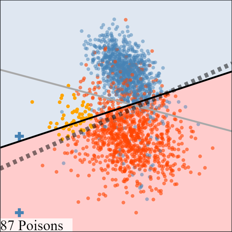
The first attack is easy for the attacker despite being against a dataset with an accurate clean model. The targeted subpopulation lies on the boundary of the cluster it belongs to, and more specifically the loss difference between the target and clean models is small. In other words, the attack causes very little "collateral damage."

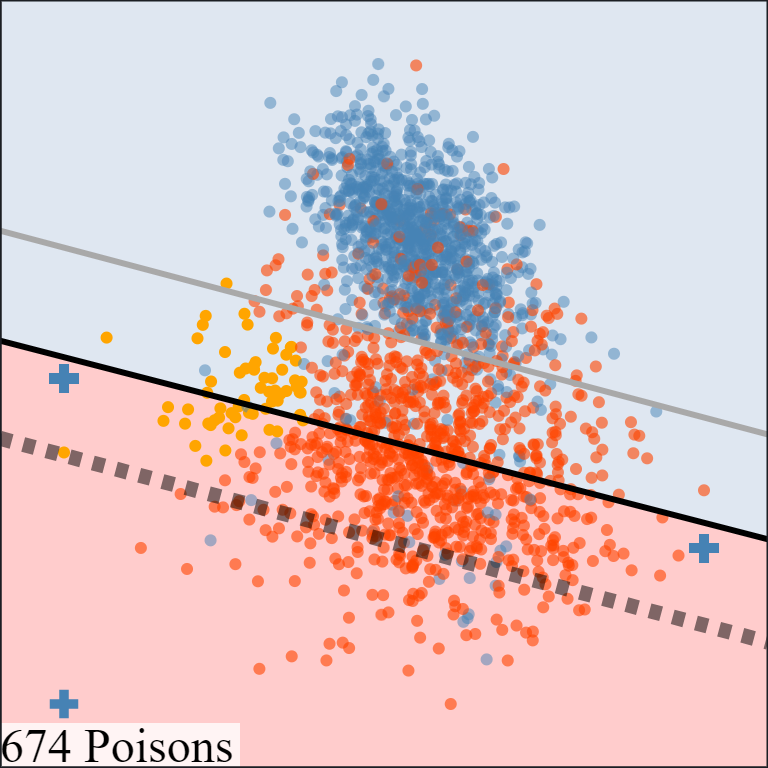
Now, consider this subpopulation in the middle of the cluster. This is our first example of an exceptionally difficult attack, requiring over 800 poisoning points. The loss difference between the target and clean models is high since the target model misclassifies a large number of points in the negative class. Notice that it seems hard even to produce a target model against this subpopulation which does not cause a large amount of collateral damage. In some sense, the subpopulation is well protected and is more robust against poisoning attacks due to its central location.

For variety, let's examine attacks against another dataset with an accurate target model.

Just as before, attack difficulty varies widely depending on the choice of subpopulation, and furthermore attack difficulty can largely be understood by examining the location of the subpopulation with respect to the rest of the dataset.

Quantitative Analysis

Visualizations are helpful, but cannot be directly created in the case of high-dimensional datasets. Now that we have visualized some of the attacks in the lower-dimensional setting, can we quantify the properties that describe the difficulty of poisoning attacks?

In the previous section, we made the observation that attack difficulty tends to increase with clean model accuracy. To be a little more precise, we can see how the attack difficulty distribution changes as a function of clean model accuracy, for our attack setup.

The histogram empirically verifies some of our observations from the earlier sections: attacks against datasets with inaccurate clean models tend to be easy, while attacks against datasets with accurate clean models can produce a wider range of attack difficulties.

Of course, on top of the general properties of the dataset and the clean model, we are more interested in knowing the properties of the subpopulation that affect attack difficulty. One way to do this is to gather a numerical description of the targeted subpopulation, and use that data to predict attack difficulty.

As expected, model loss difference strongly correlates with attack difficulty. Other numerical factors describing subpopulations, like subpopulation size, do not have clear correlations with the attack difficulty. It is possible that complex interactions among different subpopulation properties might correlate strongly with the attack difficulty, and are worth future investigations.

Adult Dataset

While the visualizations made possible by the synthetic datasets are useful for developing an intuition for subpopulation poisoning attacks, we want to understand how subpopulation susceptibility arises in a more complex and practical setting. For this purpose, we perform subpopulation poisoning attacks against the UCI Adult dataset, based on US Census data, whose associated classification task is to determine whether an adult's income exceeds $50,000 per year based on attributes such as education, age, race, and martial status.

Subpopulation Formation

Subpopulations for the Adult dataset are selected based on combinations of attributes. To generate a semantic subpopulation, first a subset of categorical features is selected, and specific values are chosen for those features. For example, the categorical features could be chosen to be "work class" and "education level", and the features' values could then be chosen to be "never worked" and "some college", respectively. Then, every negative-label ("$\le$ 50K") instance in the training set matching all of the (feature, label) pairs is extracted to form the subpopulation. The subpopulations for our experiments are chosen by considering every subset of categorical features and every combination of those features that is present in the training set. For simplicity, we only consider subpopulations with a maximum of three feature selections.

In total, 4,338 subpopulations are formed using this method. Each of these subpopulations is attacked using the same attack as in the case of synthetic dataset. Of these attacks, 1,602 were trivial (i.e., the clean model already satisfies the attack objective), leaving 2,736 nontrivial attacks.

Visualization

The Adult dataset is high-dimensional (57 dimensions after data transformations), so attacks against it cannot be directly visualized as in the case of our two-dimensional synthetic datasets. However, by employing dimensionality reduction techniques, we can indirectly visualize poisoning attacks in the high-dimensional setting.

Dimensionality reduction gives us a way to visualize the high-dimensional data in two dimensions, but we still need a way to visualize a classifier's behavior on these points. Previous attempts to visualize high-dimensional classifiers have used self-organizing maps , projection-based tour methods , hyperplane intersection techniques , or Voronoi tesslations constructed from projected data points . We will focus on another type of technique explored separately by Shulz et al. and Rodrigues et al., which attempts to produce a rich depiction of the classifier's behavior by examining the classifier's classification on data points sampled from the high-dimensional space .

The key idea is to find additional points in the high-dimensional space corresponding to points in the lower-dimensional projection space. The visualization process can be described by the following procedure:

1. Given a high-dimensional data space $\mathcal{X}$, a low-dimensional projection space $\mathcal{Z}$, and data points $x_i$ from $\mathcal{X}$, train an embedding map $\pi \colon \mathcal{X} \to \mathcal{Z}$ to obtain the projected points $z_i = \pi(x_i)$.
2. Sample the projection space $\mathcal{Z}$ to obtain the image sample points $z'_i$. Determine points $x'_i$ in the data space $\mathcal{X}$ which project to the image sample points $\pi(x'_i) \approx z_i$ via some learned inverse mapping $\pi^{-1} \colon \mathcal{Z} \to \mathcal{X}$.
3. Use the classifier $f$ defined on the data space to determine labels $f(x'_i)$ for each of the additional data points $x'_i$. Visualize the data points and classifier behavior by plotting the projected points $z_i$ on a scatterplot and coloring the background according to the sampled pairs $(z'_i, f(x'_i))$.

We apply this technique to our attacks against the Adult dataset, using Isomap embedding as our dimensionalty reduction algorithm. Here is the resulting visualization:

Already, we can see how the general behavior of the classifier changes as poisoning points are added.

The above visualization is a good way to measure the impact of poisoning points on the poisoned classifier. However, it can be difficult to see just how much the classifier's behavior is changing on the targeted subpopulation (never married). We can instead choose to perform the attack visualization technique on only the target subpopulation, in which case we get a much more focused understanding of the model's behavior:

These visualizations provide a starting point to understanding subpopulation poisoning attacks in a high-dimensional setting. But, gaining intuitions about high-dimensionality data is difficult, and any mapping to a two-dimensional space involves compromises because of our inability to display high dimensional spaces.

Quantitative Analysis

We examine the attack difficulty (measured by the ratio $p / n$) distribution of all the nontrivial attacks:

The range of difficulties as indictated by the histogram is significant: an attack with a difficulty of 0.1 uses 10 times as many points as an attack with a difficulty of 0.01. For a more concrete example, consider the subpopulation consisting of all people who have never married and the subpopulation consisting of divorced craft-repair workers (each subpopulation only taking negative-labeled instances). Both subpopulations are perfectly classified by the clean model, but the attack against the first subpopulation uses 1,490 poisoning points, while the attack against the second uses only 281.

We can also plot the attack difficulty against numerical properties of the Adult dataset subpopulations:

Semantic Subpopulation Characteristics

Recall that our goal is to determine how subpopulation characteristics affect attack difficulty. While this question can be posed in terms of the statistical properties of the subpopulation (e.g., relative size to the whole data), it is also interesting to ask which semantic properties of the subpopulation contribute significantly to the attack difficulty. In this section, we explore the relationships between attack difficulty and the semantic properties of the targeted subpopulation.

Ambient Positivity

To start, we compare a few attacks from our experiments on the Adult dataset.

The above subpopulations are all classified with 100% accuracy by the clean model and are of similar sizes (ranges from 1% to 2% of the clean training set size). So what makes some of the attacks more or less difficult? In the attacks shown above, the differences may be related to the points surrounding the subpopulation. In our experiments, we defined the subpopulations by taking only negative-label instances satisfying some semantic properties. If we remove the label restriction, we gain a more complete view of the surrounding points, and, in particular, can consider some statistics (e.g., label ratio) of the ambient points.

For a subpopulation with a given property $P$, let us call the set of all points satisfying $P$ the ambient subpopulation (since it also includes positive-label points), and call the fraction of points in the ambient subpopulation with a positive label the ambient positivity of the subpopulation. In the above attacks, attack difficulty is negatively correlated with the ambient positivity of the subpopulation. This makes sense, since positive-label points near the subpopulation work to the advantage of the attacker when attempting to induce misclassification of the negative-label points. Stated in terms of the model-targeted attack, if the clean model classifies the ambient subpopulation as the negative label, then the loss difference between the target and clean models is smaller if there are positive-label points in that region.

But does the ambient positivity of a subpopulation necessarily determine attack difficulty for otherwise similar subpopulations? If we restrict our view to subpopulations with similar pre-poisoning ambient positivity (e.g., between 0.2 and 0.3), we still find a significant spread of attack difficulties:

Once again, the above subpopulations are all classified with 100% accuracy by the clean model and are of similar sizes. Are these differences in attack difficulties just outliers due to our particular experiment setup, or is there some essential difference between the subpopulations which is not captured by their numerical descriptions? Furthermore, if such differences do exist, can they be described using the natural semantic meaning of the subpopulations?

Pairwise Analysis

What happens when two semantic subpopulations match on the same features, but differ in the value of only a single feature? For example, consider the two attacks below:

In the above example, the subpopulations possess very similar semantic descriptions, only differing in the value for the "relationship status" feature. Furthermore, the subpopulations are similarly sized with respect to the dataset (1.3% and 1.1% of the clean training set, respectively), and each subpopulation is perfectly classified by the clean model. Yet the first subpopulation required significantly more poisoning points, at least for the chosen model-targeted attack.

Adult Dataset Summary

Our experiments demonstrate that poisoning attack difficulty can vary widely, even in the simple settings we consider. Although we cannot identify all the characteristics that relate to the attack difficulty, we can characterize some of them accurately for certain groups of subpopulations, giving the first attempt in understanding this complicated problem.

Discussion

In this article, we visualize and evaluate the effectiveness of poisoning attacks, in both artificial and realistic settings. The difficulty of poisoning attacks on subpopulations varies widely, due to the properties of both the dataset and the subpopulation itself. These differences in the attack difficulty, as well as the factors that affect them, can have important consequences in understanding the realistic risks of poisoning attacks.

Our results are limited to simple settings and a linear SVM model, and it is not yet clear how well they extend to more complex models. However, as a step towards better understanding of poisoning attacks and especially in understanding how attack difficulty varies with subpopulation characteristics, experiments in such a simplified setting are valuable and revealing. Further, simple and low-capacity models are still widely used in practice due to their ease of use, low computational cost and effectiveness , and so our simplified analysis is still relevant in practice. Second, kernel methods are powerful tools to handle non-linearly separable datasets by projecting them into a linearly separable high-dimensional space and are widely adopted in practice. Therefore, if the important spatial relationships among the data points are still preserved after projection, then the same conclusions obtained in our simplified settings still apply to the more complex cases by examining the spatial relationships in the transformed space.